Как при автозаполнении будних дней исключить выходные в списке таблицы Google?
Автор: СяоянПоследнее изменение: 2017 июля 10 г.
В Microsoft Excel мы можем легко заполнить только будние дни и исключить выходные с помощью параметров автозаполнения. Но в таблице Google нет возможности заполнять будние дни так быстро, как в Excel. Как бы вы справились с этой задачей в листе Google?
В таблице Google вы можете применить следующую формулу для заполнения будних дней только по мере необходимости.
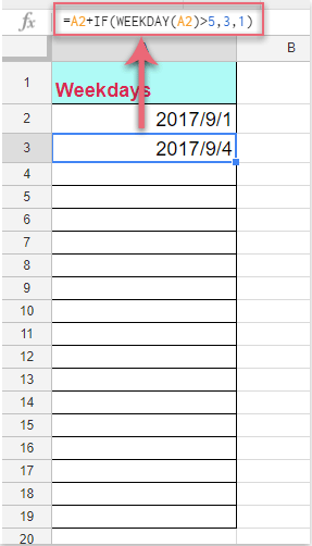
1. Введите первую дату, которую вы хотите начать, а затем введите эту формулу под первой ячейкой даты: = A2 + ЕСЛИ (ДЕНЬ НЕДЕЛИ (A2)> 5,3,1), см. снимок экрана:
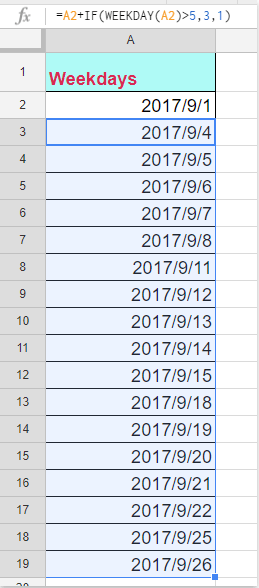
2, нажмите Enter а затем перетащите дескриптор заполнения вниз к ячейкам, которые вы хотите заполнить буднями, и только последовательные дни недели заполняются в столбце, как показано на следующем снимке экрана:
Улучшите свои навыки работы с Excel с помощью Kutools for Excel и почувствуйте эффективность, как никогда раньше. Kutools for Excel предлагает более 300 расширенных функций для повышения производительности и экономии времени. Нажмите здесь, чтобы получить функцию, которая вам нужна больше всего...
This comment was minimized by the moderator on the site
how to insert holidays here? Say for example, in India we have 26th January, 15th August and 2nd October as holidays. How do i avoid these dates in the autofill?
This comment was minimized by the moderator on the site
how to insert holidays here? Say for example, in India we have 26th January, 15th August and 2nd October as holidays. How do i avoid these dates in the autofill?
This comment was minimized by the moderator on the site
This is super helpful. Would you be able to give a little more information about how to manipulate this formula? For example, I only want to fill Mondays and Wednesdays. Is this possible?
This comment was minimized by the moderator on the site
Hi, Clayton,
To only fill Mondays and Wednesdays into a list of cells, you should do as this:
First, enter the date which is Monday or Wednesday in cell A1, and then copy the below formula into cell A2, then drag the fill handle down to your need:
=IF(TEXT(A1,"ddd")="Mon",A1+2,A1+5)
This comment was minimized by the moderator on the site
Is it possible to use this with an arrayformula across a horizontal row? I tried it but having some issues.
=arrayformula(if(COLUMN(C13:Z13), IF(INDIRECT(ADDRESS(ROW(C13:Z13),COLUMN(C13:Z13)-1)), INDIRECT(ADDRESS(ROW(C13:Z13),COLUMN(C13:Z13)-1)) + IF(WEEKDAY(INDIRECT(ADDRESS(ROW(C13:Z13),COLUMN(C13:Z13)-1)))>5,3,1), -1
) , -2))

")
")