Вернуть несколько совпадающих значений на основе нескольких критериев в Excel (Полное руководство)
Пользователи Excel часто сталкиваются с ситуациями, когда необходимо извлечь несколько значений, удовлетворяющих нескольким условиям одновременно, и представить все совпадающие результаты в столбце, строке или объединить в одной ячейке. Это руководство рассматривает методы для всех версий Excel, а также новую функцию FILTER, доступную в Excel 365 и 2021.
Вернуть несколько совпадающих значений на основе нескольких критериев в одной ячейке
В Excel извлечение нескольких совпадающих значений на основе множественных критериев внутри одной ячейки является распространенной задачей. Здесь рассмотрены два эффективных метода.
Метод 1: Использование функции TEXTJOIN (Excel365 / 2021, 2019)
Чтобы получить все совпадающие значения в одну ячейку с разделителями, функция TEXTJOIN может помочь.
Введите или скопируйте следующую формулу в пустую ячейку, затем нажмите клавишу Enter (Excel 2021 и Excel 365) или Ctrl + Shift + Enter в Excel 2019, чтобы получить результат:
=TEXTJOIN(", ", TRUE, IF(($A$2:$A$18=E2)*($B$2:$B$18=F2), $C$2:$C$18, ""))
- ($A$2:$A$21=E2)*($B$2:$B$21=F2) проверяет, соответствует ли каждая строка обоим условиям: «Продавец равен E2» и «Месяц равен F2». Если оба условия выполнены, результат равен 1; в противном случае — 0. Звездочка * означает, что оба условия должны быть истинными.
- IF(..., $C$2:$C$21, "") возвращает название продукта, если строка совпадает; в противном случае возвращает пустое значение.
- TEXTJOIN(", ", TRUE, ...) объединяет все непустые названия продуктов в одну ячейку, разделяя их запятой «, ».
Метод 2: Использование Kutools для Excel
Kutools для Excel предлагает мощное, но простое решение, позволяющее быстро получить и объединить несколько совпадений в одну ячейку на основе множественных критериев без сложных формул.
После установки Kutools для Excel выполните следующие действия:
- Выберите диапазон данных, по которому вы хотите получить все соответствующие значения на основе критериев.
- Затем нажмите Kutools > Объединить и Разделить > Расширенное объединение строк, см. скриншот:

- В диалоговом окне Расширенное объединение строк настройте следующие параметры:
- Выберите заголовки столбцов, содержащих ваши критерии совпадения (например, Продавец и Месяц). Для каждого выбранного столбца нажмите Основной ключ, чтобы определить их как условия поиска.
- Нажмите заголовок столбца, где вы хотите получить объединенные результаты (например, Продукт). Из раздела Объединить выберите предпочитаемый разделитель (например, запятую, пробел или пользовательский разделитель).
- В конце нажмите кнопку OK.


Результат: Kutools мгновенно объединит все совпадающие значения в одну ячейку для каждой уникальной комбинации критериев.

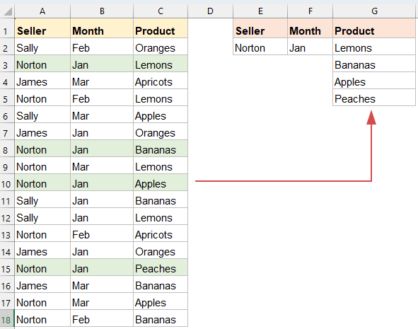
Вернуть несколько совпадающих значений на основе нескольких критериев в столбец
Когда вам нужно извлечь и отобразить несколько совпадающих записей из набора данных на основе нескольких условий, возвращая результаты в вертикальном формате столбца, Excel предлагает несколько мощных решений.
Метод 1: Использование формулы массива (для всех версий)
Вы можете использовать следующую формулу массива для возврата результатов вертикально в столбец:
1. Скопируйте или введите следующую формулу в пустую ячейку:
=IFERROR(INDEX($C$2:$C$18, SMALL(IF(($A$2:$A$18=$E$2)*($B$2:$B$18=$F$2), ROW($C$2:$C$18)-ROW($C$2)+1), ROW(1:1))), "")2. Нажмите Ctrl + Shift + Enter, чтобы получить первое совпадение, затем выберите первую ячейку с формулой и протяните маркер заполнения вниз до тех пор, пока не появится пустая ячейка. Теперь все совпадающие значения возвращены, как показано на скриншоте ниже:

- $A$2:$A$18=$E$2: Проверяет, совпадает ли Продавец со значением в ячейке E2.
- $B$2:$B$18=$F$2: Проверяет, совпадает ли Месяц со значением в ячейке F2.
- * является логическим оператором И (оба условия должны быть истинными).
- ROW($C$2:$C$18)-ROW($C$2)+1: Генерирует относительный номер строки для каждого продукта.
- SMALL(..., ROW(1:1)): Получает n-е наименьшее совпадающее значение (по мере того, как формула тянется вниз).
- INDEX(...): Возвращает продукт из совпадающей строки.
- IFERROR(..., ""): Возвращает пустую ячейку, если больше нет совпадений.
Метод 2: Использование функции FILTER (Excel365 / 2021)
Если вы используете Excel 365 или Excel 2021, функция FILTER является отличным выбором для возврата нескольких результатов на основе нескольких критериев благодаря своей простоте, ясности и способности динамически выводить результаты без сложных формул массива.
Скопируйте или введите приведенную ниже формулу в пустую ячейку, затем нажмите клавишу Enter, и все совпадающие записи будут возвращены на основе нескольких критериев.
=FILTER(C2:C18, (A2:A18=E2)*(B2:B18=F2), "No match")
- FILTER(...) возвращает все значения из C2:C18, где выполнены оба условия.
- (A2:A18=E2)*(B2:B18=F2): Логический массив, который проверяет совпадающего продавца и месяц.
- "No match": Необязательное сообщение, если значения не найдены.
Вернуть несколько совпадающих значений на основе нескольких критериев в строку
Пользователи Excel часто нуждаются в извлечении нескольких значений из набора данных, которые соответствуют нескольким условиям и отображении их горизонтально (в строке). Это полезно для создания динамических отчетов, панелей управления или сводных таблиц, где ограничено вертикальное пространство. В этом разделе мы рассмотрим два мощных метода.
Метод 1: Использование формулы массива (для всех версий)
Традиционные формулы массива позволяют извлекать несколько совпадающих значений с использованием функций INDEX, SMALL, IF и COLUMN. В отличие от вертикального извлечения (основанного на столбце), мы адаптируем формулу для возврата результатов в строке.
1. Скопируйте или введите приведенную ниже формулу в пустую ячейку:
=IFERROR(INDEX($C$2:$C$18, SMALL(IF(($A$2:$A$18=$E$2)*($B$2:$B$18=$F$2), ROW($C$2:$C$18)-ROW($C$2)+1), COLUMN(A1))), "")2. Нажмите Ctrl + Shift + Enter для получения первого совпадающего результата, затем выберите первую ячейку с формулой и протяните формулу вправо по столбцам для получения всех результатов.

- $A$2:$A$18=$E$2: Проверяет, совпадает ли Продавец.
- $B$2:$B$18=$F$2: Проверяет, совпадает ли Месяц.
- *: Логическое И — оба условия должны быть истинными.
- ROW($C$2:$C$18)-ROW($C$2)+1: Создает относительные номера строк.
- COLUMN(A1): Корректирует, какое совпадение возвращать, в зависимости от того, насколько далеко формула была протянута вправо.
- IFERROR(...): Предотвращает ошибки после исчерпания совпадений.
Метод 2: Использование функции FILTER (Excel365 / 2021)
Скопируйте или введите приведенную ниже формулу в пустую ячейку, затем нажмите клавишу Enter, и все совпадающие значения будут извлечены и расположены в строке. См. скриншот:
=TRANSPOSE(FILTER(C2:C18, (A2:A18=E2)*(B2:B18=F2), "No match"))
- FILTER(...): Извлекает совпадающие значения из столбца C на основе двух условий.
- (A2:A18=E2)*(B2:B18=F2): Оба условия должны быть истинными.
- TRANSPOSE(...): Преобразует вертикальный массив, возвращаемый FILTER, в горизонтальный массив.
🔚 Заключение
Извлечение нескольких совпадающих значений на основе нескольких критериев в Excel может быть выполнено несколькими способами, в зависимости от того, как вы хотите отобразить результаты — будь то в столбце, строке или в пределах одной ячейки.
- Для пользователей с Excel 365 или Excel 2021 функция FILTER предлагает современное, динамичное и элегантное решение, которое минимизирует сложность.
- Для тех, кто использует более старые версии, формулы массива остаются мощными инструментами, хотя требуют немного больше настройки и внимания.
- Кроме того, если вы хотите объединить результаты в одну ячейку или предпочитаете решение без кода, функция TEXTJOIN или сторонние инструменты, такие как Kutools для Excel, могут значительно упростить процесс.
Выберите метод, который лучше всего подходит для вашей версии Excel и вашей предпочтительной компоновки, и вы будете хорошо подготовлены для эффективного и точного выполнения поисков по нескольким критериям. Если вас интересует изучение дополнительных советов и приемов Excel, наш веб-сайт предлагает тысячи учебных материалов, чтобы помочь вам освоить Excel.
Больше связанных статей:
- Вернуть несколько значений поиска в одну ячейку, разделенную запятыми
- В Excel мы можем применить функцию VLOOKUP, чтобы вернуть первое совпадающее значение из таблицы, но иногда нам нужно извлечь все совпадающие значения, а затем разделить их конкретным разделителем, например запятой, тире и т.д., в одну ячейку, как показано на следующем скриншоте. Как можно получить и вернуть несколько значений поиска в одну ячейку, разделенную запятыми, в Excel?
- Vlookup и вернуть несколько совпадающих значений сразу в Google Таблицах
- Обычная функция Vlookup в Google Таблицах может помочь найти и вернуть первое совпадающее значение на основе заданных данных. Но иногда вам может понадобиться выполнить vlookup и вернуть все совпадающие значения, как показано на следующем скриншоте. Есть ли у вас хорошие и простые способы решить эту задачу в Google Таблицах?
- Vlookup и вернуть несколько значений из выпадающего списка
- В Excel, как вы можете выполнить vlookup и вернуть несколько соответствующих значений из выпадающего списка, что означает, что при выборе одного элемента из выпадающего списка отображаются все его связанные значения сразу, как показано на следующем скриншоте. В этой статье я покажу решение пошагово.
- Vlookup и вернуть несколько значений вертикально в Excel
- Обычно вы можете использовать функцию Vlookup, чтобы получить первое соответствующее значение, но иногда вы хотите вернуть все совпадающие записи на основе определенного критерия. В этой статье я расскажу, как выполнить vlookup и вернуть все совпадающие значения вертикально, горизонтально или в одну ячейку.
- Vlookup и вернуть совпадающие данные между двумя значениями в Excel
- В Excel мы можем применить обычную функцию Vlookup, чтобы получить соответствующее значение на основе заданных данных. Но иногда мы хотим выполнить vlookup и вернуть совпадающее значение между двумя значениями, как показано на следующем скриншоте. Как вы можете справиться с этой задачей в Excel?
Лучшие инструменты для повышения продуктивности в Office
Повысьте свои навыки работы в Excel с помощью Kutools для Excel и ощутите эффективность на новом уровне. Kutools для Excel предлагает более300 расширенных функций для повышения производительности и экономии времени. Нажмите здесь, чтобы выбрать функцию, которая вам нужнее всего...
Office Tab добавляет вкладки в Office и делает вашу работу намного проще
- Включите режим вкладок для редактирования и чтения в Word, Excel, PowerPoint, Publisher, Access, Visio и Project.
- Открывайте и создавайте несколько документов во вкладках одного окна вместо новых отдельных окон.
- Увеличьте свою продуктивность на50% и уменьшите количество щелчков мышью на сотни ежедневно!
Все надстройки Kutools. Один установщик
Пакет Kutools for Office включает надстройки для Excel, Word, Outlook и PowerPoint, а также Office Tab Pro — идеально для команд, работающих в разных приложениях Office.
- Комплексный набор — надстройки для Excel, Word, Outlook и PowerPoint плюс Office Tab Pro
- Один установщик, одна лицензия — настройка занимает считанные минуты (MSI-совместимо)
- Совместная работа — максимальная эффективность между приложениями Office
- 30-дневная полнофункциональная пробная версия — без регистрации и кредитной карты
- Лучшее соотношение цены и качества — экономия по сравнению с покупкой отдельных надстроек