Как выполнить условное форматирование на основе другого листа в Google Таблицах?
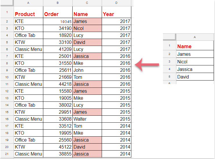
Условное форматирование — это полезная функция в Google Таблицах, которая позволяет автоматически выделять ячейки на основе определенных критериев, что упрощает анализ и визуализацию данных. Иногда вместо выделения ячеек в соответствии со значениями на том же листе может потребоваться, чтобы правила форматирования основывались на списке или критериях, хранящихся на другом листе. Например, можно выделить ячейки на одном листе, которые также появляются в списке, поддерживаемом на другом листе, как показано на скриншоте ниже. Такие задачи распространены при работе с перекрестными ссылками на данные, например, при сравнении текущих продаж с основным списком продуктов или проверке на наличие дубликатов из другого источника данных. Однако настройка такого условного форматирования в Google Таблицах, особенно при обращении к данным на разных листах, может быть запутанной, если вы раньше этого не делали. Руководство ниже покажет вам пошаговый простой подход для достижения этой цели.
Условное форматирование для выделения ячеек на основе списка из другого листа в Google Таблицах
Условное форматирование для выделения ячеек на основе списка из другого листа в Google Таблицах
Этот метод позволяет настроить правило условного форматирования для выделения ячеек на активном листе, если они присутствуют в указанном списке с другого листа. Такое межлистовое условное форматирование особенно полезно для динамического отслеживания данных и поддержания согласованности между связанными наборами данных.
Чтобы завершить этот процесс, следуйте этим подробным шагам:
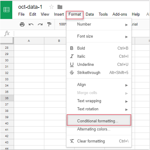
1. Откройте целевой рабочий лист, затем нажмите меню Формат в верхней части экрана и выберите Условное форматирование. Панель Правила условного форматирования откроется с правой стороны экрана.
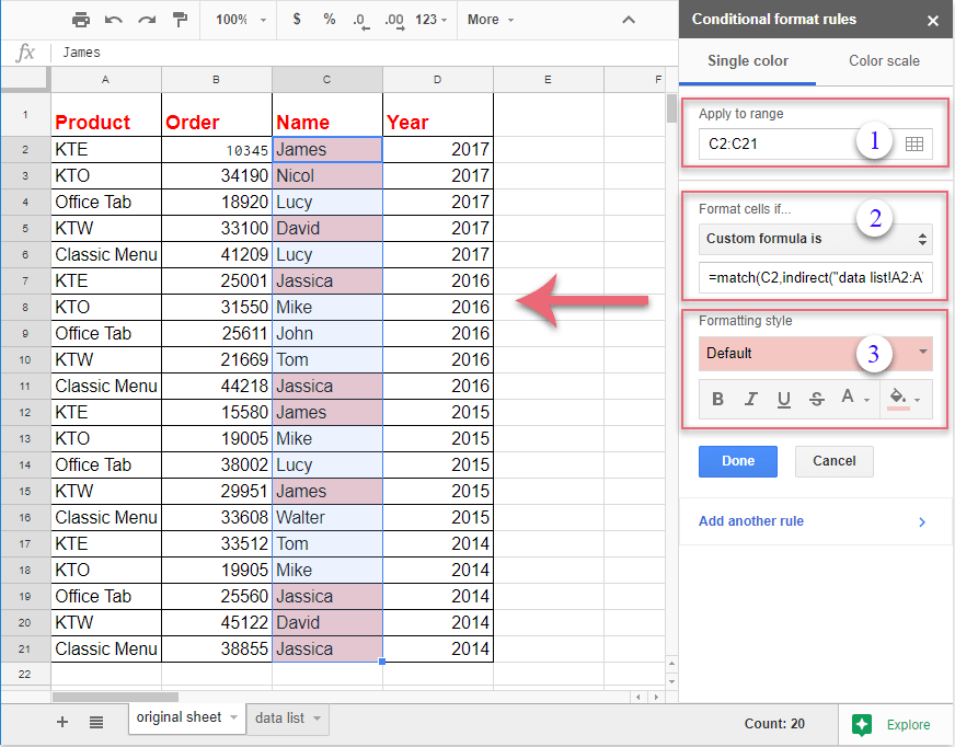
2. На панели Правила условного форматирования выполните следующие действия:
(1.) Нажмите кнопку ![]() рядом с полем «Применить к диапазону». Выберите диапазон ячеек, которые вы хотите выделить. Например, если вы хотите отформатировать все значения в столбце C, начиная со строки 2, выберите C2:C. Выбор подходящего диапазона гарантирует, что только нужные ячейки будут оцениваться для форматирования.
рядом с полем «Применить к диапазону». Выберите диапазон ячеек, которые вы хотите выделить. Например, если вы хотите отформатировать все значения в столбце C, начиная со строки 2, выберите C2:C. Выбор подходящего диапазона гарантирует, что только нужные ячейки будут оцениваться для форматирования.
(2.) В раскрывающемся меню «Форматировать ячейки, если» выберите Пользовательская формула. Введите следующую формулу в предоставленное поле: =match(C2,indirect("data list!A2:A"),0). Эта формула проверяет, соответствует ли каждая ячейка в столбце C любому значению в диапазоне A2:A листа «data list».
(3.) В разделе Стиль форматирования выберите желаемый формат, например, заливку ячейки определенным цветом или изменение стиля шрифта. Вы можете сразу просмотреть стиль в вашем листе перед его применением.
Примечание: В приведенной выше формуле C2 относится к первой ячейке вашего выбранного диапазона (настройте, если ваши данные начинаются в другой строке или столбце), а data list!A2:A указывает на имя листа («data list») и соответствующий диапазон (A2:A), где хранится ваш список с другого листа. Убедитесь, что ссылка на ячейку в формуле соответствует левому верхнему углу выбранного диапазона, иначе форматирование может не примениться правильно. Если ваш диапазон другого списка отличается, обязательно обновите его в формуле (например, «data list!B2:B»).
3. После настройки правила совпадающие ячейки в выбранном диапазоне будут мгновенно выделены на основе списка с другого листа. Просмотрите предварительный просмотр, затем нажмите Готово в нижней части панели Правила условного форматирования, чтобы применить и сохранить форматирование.
Советы и устранение неполадок:
- Тщательно проверьте формулу на наличие опечаток, особенно в именах листов и ссылках на диапазон — неправильные ссылки являются частой причиной того, что правила не применяются.
- Если ваш список данных содержит пустые ячейки, функция
MATCHвернет ошибку#N/Aдля несоответствующих значений, но это ожидаемое поведение и не влияет на выделение совпадающих элементов. - Когда вы копируете форматирование на новый лист или изменяете диапазоны, убедитесь, что вы также обновили ссылки на ячейки в своей пользовательской формуле соответственно.
- Форматирование обновляется автоматически, если вы позже добавляете или удаляете элементы из вашего списка ссылок.
- Лист и диапазон, указанные в вашей формуле, существуют и написаны правильно.
- Первая ячейка в вашей формуле соответствует первой ячейке выбранного диапазона.
- Все необходимые разрешения для доступа между листами в вашей таблице доступны — этот метод работает внутри одного файла Google Таблиц с несколькими листами, но не между разными файлами.
В качестве альтернативы, если структура ваших данных или требования более сложные — например, если вам нужно сравнивать несколько столбцов, допускать частичные совпадения или выполнять более сложные операции поиска — использование вспомогательных столбцов с формулами COUNTIF или VLOOKUP, или использование Google Apps Script (пользовательский JavaScript-код), также может обеспечить гибкие решения для условного форматирования.
Подводя итог, настройка условного форматирования на основе другого листа крайне эффективна для проверки списков, отслеживания дубликатов и различных межлистовых проверок данных — всё это внутри Google Таблиц. Всегда убедитесь, что ваши входные данные формул, ссылочные диапазоны и правила форматирования настроены для получения плавных и точных результатов.

Раскройте магию Excel с Kutools AI
- Умное выполнение: Выполняйте операции с ячейками, анализируйте данные и создавайте диаграммы — всё это посредством простых команд.
- Пользовательские формулы: Создавайте индивидуальные формулы для оптимизации ваших рабочих процессов.
- Кодирование VBA: Пишите и внедряйте код VBA без особых усилий.
- Интерпретация формул: Легко разбирайтесь в сложных формулах.
- Перевод текста: Преодолейте языковые барьеры в ваших таблицах.
Лучшие инструменты для повышения продуктивности в Office
Повысьте свои навыки работы в Excel с помощью Kutools для Excel и ощутите эффективность на новом уровне. Kutools для Excel предлагает более300 расширенных функций для повышения производительности и экономии времени. Нажмите здесь, чтобы выбрать функцию, которая вам нужнее всего...
Office Tab добавляет вкладки в Office и делает вашу работу намного проще
- Включите режим вкладок для редактирования и чтения в Word, Excel, PowerPoint, Publisher, Access, Visio и Project.
- Открывайте и создавайте несколько документов во вкладках одного окна вместо новых отдельных окон.
- Увеличьте свою продуктивность на50% и уменьшите количество щелчков мышью на сотни ежедневно!
Все надстройки Kutools. Один установщик
Пакет Kutools for Office включает надстройки для Excel, Word, Outlook и PowerPoint, а также Office Tab Pro — идеально для команд, работающих в разных приложениях Office.
- Комплексный набор — надстройки для Excel, Word, Outlook и PowerPoint плюс Office Tab Pro
- Один установщик, одна лицензия — настройка занимает считанные минуты (MSI-совместимо)
- Совместная работа — максимальная эффективность между приложениями Office
- 30-дневная полнофункциональная пробная версия — без регистрации и кредитной карты
- Лучшее соотношение цены и качества — экономия по сравнению с покупкой отдельных надстроек