Как создать динамический выпадающий список в Google Sheets?
Вставка обычного выпадающего списка в Google Sheets может быть для вас простой задачей, но иногда вам может понадобиться создать динамический выпадающий список, где второй список зависит от выбора в первом списке. Как можно справиться с этой задачей в Google Sheets?
Создание динамического выпадающего списка в Google Sheets
Создание динамического выпадающего списка в Google Sheets
Выполните следующие шаги, чтобы создать динамический выпадающий список в Google Sheets:
1. Сначала вы должны вставить базовый выпадающий список, пожалуйста, выберите ячейку, куда вы хотите поместить первый выпадающий список, а затем нажмите Данные > Проверка данных, см. скриншот:

2. В появившемся диалоговом окне Проверка данных выберите Список из диапазона из выпадающего списка рядом с разделом Критерии , а затем нажмите ![]() кнопку, чтобы выбрать значения ячеек, на основе которых вы хотите создать первый выпадающий список, см. скриншот:
кнопку, чтобы выбрать значения ячеек, на основе которых вы хотите создать первый выпадающий список, см. скриншот:

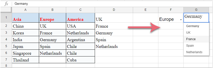
3. Затем нажмите кнопку Сохранить, и первый выпадающий список будет создан. Выберите один элемент из созданного выпадающего списка, а затем введите эту формулу: =arrayformula(if(F1=A1,A2:A7,if(F1=B1,B2:B6,if(F1=C1,C2:C7,"")))) в пустую ячейку, которая находится рядом с колонками данных, затем нажмите клавишу Enter, все соответствующие значения на основе элемента первого выпадающего списка будут отображены сразу, см. скриншот:
Примечание: В приведенной выше формуле: F1 — это ячейка первого выпадающего списка, A1, B1 и C1 — это элементы первого выпадающего списка, A2:A7, B2:B6 и C2:C7 — это значения ячеек, на основе которых создается второй выпадающий список. Вы можете изменить их на свои собственные.

4. После этого вы можете создать второй зависимый выпадающий список, щелкните ячейку, куда вы хотите поместить второй выпадающий список, а затем нажмите Данные > Проверка данных, чтобы перейти в диалоговое окно Проверка данных, выберите Список из диапазона из выпадающего списка рядом с разделом Критерии, и продолжайте нажимать кнопку, чтобы выбрать ячейки с формулами, которые являются результатами соответствия элементу первого выпадающего списка, см. скриншот:

5. Наконец, нажмите кнопку Сохранить, и второй зависимый выпадающий список будет успешно создан, как показано на следующем скриншоте:
Лучшие инструменты для повышения продуктивности в Office
Повысьте свои навыки работы в Excel с помощью Kutools для Excel и ощутите эффективность на новом уровне. Kutools для Excel предлагает более300 расширенных функций для повышения производительности и экономии времени. Нажмите здесь, чтобы выбрать функцию, которая вам нужнее всего...
Office Tab добавляет вкладки в Office и делает вашу работу намного проще
- Включите режим вкладок для редактирования и чтения в Word, Excel, PowerPoint, Publisher, Access, Visio и Project.
- Открывайте и создавайте несколько документов во вкладках одного окна вместо новых отдельных окон.
- Увеличьте свою продуктивность на50% и уменьшите количество щелчков мышью на сотни ежедневно!
Все надстройки Kutools. Один установщик
Пакет Kutools for Office включает надстройки для Excel, Word, Outlook и PowerPoint, а также Office Tab Pro — идеально для команд, работающих в разных приложениях Office.
- Комплексный набор — надстройки для Excel, Word, Outlook и PowerPoint плюс Office Tab Pro
- Один установщик, одна лицензия — настройка занимает считанные минуты (MSI-совместимо)
- Совместная работа — максимальная эффективность между приложениями Office
- 30-дневная полнофункциональная пробная версия — без регистрации и кредитной карты
- Лучшее соотношение цены и качества — экономия по сравнению с покупкой отдельных надстроек