Перейти к основному содержанию

Как найти n-ю непустую ячейку в Excel?

Как вы могли найти и вернуть n-е непустое значение ячейки из столбца или строки в Excel? В этой статье я расскажу о некоторых полезных формулах для решения этой задачи.

Найдите и верните n-е непустое значение ячейки из столбца с формулой

Найти и вернуть n-е непустое значение ячейки из строки с формулой


стрелка синий правый пузырь Найдите и верните n-е непустое значение ячейки из столбца с формулой

Например, у меня есть столбец данных, как показано на следующем снимке экрана, теперь я получу третье непустое значение ячейки из этого списка.

doc найти n-й непустой 1

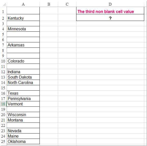
Пожалуйста, введите эту формулу: =INDEX($A$1:$A$25,SMALL(ROW($A$1:$A$25)+(100*($A$1:$A$25="")), 3))&"" в пустую ячейку, в которую вы хотите вывести результат, например, D2, а затем нажмите Shift + Ctrl + Enter вместе, чтобы получить правильный результат, см. снимок экрана:

doc найти n-й непустой 2

Внимание: В формуле выше A1: A25 это список данных, который вы хотите использовать, и номер 3 указывает на третье непустое значение ячейки, которое вы хотите вернуть, если вы хотите получить вторую непустую ячейку, вам просто нужно изменить число 3 на 2, как вам нужно.


стрелка синий правый пузырь Найти и вернуть n-е непустое значение ячейки из строки с формулой

Если вы хотите найти и вернуть n-е непустое значение ячейки в строке, вам может помочь следующая формула, сделайте следующее:

Введите эту формулу: =INDEX($A$1:$M$1,SMALL(IF($A$1:$M$1<>"",COLUMN($A$1:$M$1)-COLUMN($A$1)+1),4)) в пустую ячейку, где вы хотите найти результат, а затем нажмите Shift + Ctrl + Enter ключи вместе, чтобы получить результат, см. снимок экрана:

doc найти n-й непустой 3

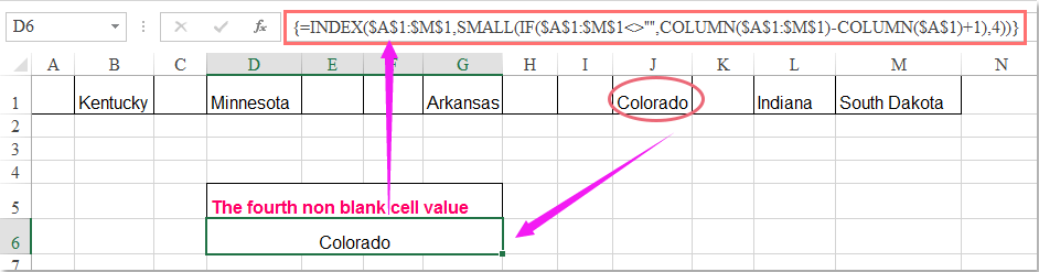
Примечание: В приведенной выше формуле A1: M1 - это значения строки, которые вы хотите использовать, а число 4 - это четвертое непустое значение ячейки, которое вы хотите вернуть, если вы хотите получить вторую непустую ячейку, вам просто нужно изменить число 4 на 2, как вам нужно.

Лучшие инструменты для офисной работы

🤖 Kutools AI Помощник: Революционный анализ данных на основе: Интеллектуальное исполнение   |  Генерировать код  |  Создание пользовательских формул  |  Анализ данных и создание диаграмм  |  Вызов функций Kutools...
Популярные опции: Найдите, выделите или определите дубликаты   |  Удалить пустые строки   |  Объедините столбцы или ячейки без потери данных   |   Раунд без формулы ...
Супер поиск: Множественный критерий VLookup    VLookup с несколькими значениями  |   VLookup по нескольким листам   |   Нечеткий поиск ....
Расширенный раскрывающийся список: Быстрое создание раскрывающегося списка   |  Зависимый раскрывающийся список   |  Выпадающий список с множественным выбором ....
Менеджер столбцов: Добавить определенное количество столбцов  |  Переместить столбцы  |  Переключить статус видимости скрытых столбцов  |  Сравнить диапазоны и столбцы ...
Рекомендуемые функции: Сетка Фокус   |  Просмотр дизайна   |   Большой Формулный Бар    Менеджер книг и листов   |  Библиотека ресурсов (Авто текст)   |  Выбор даты   |  Комбинировать листы   |  Шифровать/дешифровать ячейки    Отправлять электронные письма по списку   |  Суперфильтр   |   Специальный фильтр (фильтровать жирным шрифтом/курсивом/зачеркиванием...) ...
15 лучших наборов инструментов12 Текст Инструменты (Добавить текст, Удалить символы, ...)   |   50+ График Тип (Диаграмма Ганта, ...)   |   40+ Практических Формулы (Рассчитать возраст по дню рождения, ...)   |   19 Вносимые Инструменты (Вставить QR-код, Вставить изображение из пути, ...)   |   12 Конверсия Инструменты (Числа в слова, Конверсия валюты, ...)   |   7 Слияние и разделение Инструменты (Расширенные ряды комбинирования, Разделить клетки, ...)   |   ... и более

Улучшите свои навыки работы с Excel с помощью Kutools for Excel и почувствуйте эффективность, как никогда раньше. Kutools for Excel предлагает более 300 расширенных функций для повышения производительности и экономии времени.  Нажмите здесь, чтобы получить функцию, которая вам нужна больше всего...

Описание


Вкладка Office: интерфейс с вкладками в Office и упрощение работы

  • Включение редактирования и чтения с вкладками в Word, Excel, PowerPoint, Издатель, доступ, Visio и проект.
  • Открывайте и создавайте несколько документов на новых вкладках одного окна, а не в новых окнах.
  • Повышает вашу продуктивность на 50% и сокращает количество щелчков мышью на сотни каждый день!
Comments (10)
No ratings yet. Be the first to rate!
This comment was minimized by the moderator on the site
CIAO STO CERCANDO DI APPLICARE LA TUA FORMULA MA NON MI FUNZIONA, DOVE STO SBAGLIANDO?
=INDICE($K$37:$K$88;MIN(RIGHE($K$37:$K$88)+RIGHE(100*($K$37:$K$88=""));6))&""
DEVO VISUALIZZARE L'ENNESIMA RIGA DIVERSA DA VUOTO

GRAzie
This comment was minimized by the moderator on the site
=INDICE($K$37:$K$88;MIN(RIGHE($K$37:$K$88)+(100*($K$37:$K$88=""));6))&""
This comment was minimized by the moderator on the site
I'm running this formula on a ~400 row sheet with around 20 blanks mixed throughout the data, and it's working perfectly EXCEPT when I fill the series down, it sometimes duplicates a row for some reason. For example, it seems to think a value is somehow simultaneously the 331st non-blank and the 332nd.

Things I've noticed:
-Duplications always happen in pairs (ex. 331 and 332 are duplicates, 333 and 334 will also be), then it goes back to normal for a while.
-Raw data also has blanks in pairs, but not corresponding to the duplicates
-No duplications occur in the first 94 rows, but they happen every 33-35 rows after that
-Does not appear to be linked to the value in the cell being duplicated
-I have entered as an array and as a standard formula, no difference in function

For reference, here's my actual formula:

=INDEX('PO Raw Data'!CR:CR,SMALL(ROW('PO Raw Data'!CR:CR)+(100*('PO Raw Data'!CR:CR="")),$W2)&"")

Note $W2 refers to a helper column and counts up as the data set is filled down, but only because I couldn't get it to count up when I just used a number instead of cell reference.
When I've replaced that cell reference (ex. $W2) with the appropriate number, same result.


Any thoughts on what I can do to fix that?
This comment was minimized by the moderator on the site
very helpful,
although when I return the nth non blank cell in a column set to DATE, the returned value appears as number(general number).formatting the cell into DATE also doesn't change the result. could you please give me a hand!
thanks a lot
This comment was minimized by the moderator on the site
Hello, Shirazi,
Sorry, maybe there is no direct formula for you to get the date format.

If someone else has the solution, please comment here.
This comment was minimized by the moderator on the site
Hi everyone!


Could you also help me return the row number of the second, third non-blank cell?


Please help me.
This comment was minimized by the moderator on the site
Hello, John,
the following formula can help you to get all the row numbers of the non-blank cells, please try it, thank you!
=IFERROR(ROW(INDEX($A$1:$A$12,SMALL(INDEX(NOT(ISBLANK($A$1:$A$12))*ROW($A$1:$A$12),0),COUNTBLANK($A$1:$A$12)+ROW(A1)))),"")
This comment was minimized by the moderator on the site
Hey everyone,

I have a table with numerous columns and rows. The rows have range names, and a description/location at the beginning of the row range with its own range, example "Building No.s". There are multiple Row Ranges/ Buildings. There are headers at the top of each columns for specific "Building Assembly Types". The table content is numeric quantities for each type "Building Assembly Type" for each specific "Building" description/location. There could be as many as (100) "Building Assembly Types" column headers but I will limit the assemblies to (10) per row range, so there will be numerous blank cells in each "Building No." range.

I have other summary tables set up for each "Building" that I want to pull the non-blank cells quantities to, along with the corresponding header "Assembly Type" for each "Building" with a (10) max "Assemblies" per page.

I can identify the non-blank cell quantities by use of the array formula above for rows. The problem I am having is identifying the header that corresponds to it.

Ultimately if I can identify the "Assembly" header, I can always index the "Quantities" once I have the header "Assembly" identified for each "Building". Then I would be able do a lookup for all the parts associated with each "Assembly" type for that "Building" from my Assembly parts database and multiply it times the "Quantity" of each assembly type.

Hopefully this makes since and someone can help.
This comment was minimized by the moderator on the site
Hello, I am looking for the third blank row in a column and I copied your formula and just changed the range from $A$1:$A:$25 to my range $D$306:$D$354. But when I change the range I get #REF! as my answer. I already converted to an array, control-shift-enter. Now the cell range I am referencing has formulas in them, so could that be why I am getting #REF. Your formula: =INDEX($A$1:$A$25,SMALL(ROW($A$1:$A$25)+(100*($A$1:$A$25="")), 3))&"" My formula: =INDEX($D$306:$D$354,SMALL(ROW($D$306:$D$354)+(1*($D$306:$D$354="")), 2))&"" Thanks, Noel
This comment was minimized by the moderator on the site
you have put the 1 instead of 100 therefore answered was wrong. please use below formula

INDEX($D$306:$D$354,SMALL(ROW($D$306:$D$354)+(100*($D$306:$D$354="")), 3))&"" than ctrl + shift+enter
There are no comments posted here yet
Please leave your comments in English
Posting as Guest
×
Rate this post:
0   Characters
Suggested Locations