Как создать выпадающий список с несколькими флажками в Excel?
Традиционные выпадающие списки в Excel ограничивают пользователей одиночным выбором. Чтобы преодолеть это ограничение и позволить множественный выбор, мы рассмотрим два практических метода создания выпадающих списков с несколькими флажками.
Используйте Поле со списком для создания выпадающего списка с несколькими флажками
A: Создайте поле со списком с исходными данными
B: Назовите ячейку, в которой будут находиться выбранные элементы
C: Вставьте фигуру для вывода выбранных элементов
Легко создавайте выпадающий список с флажками с помощью удивительного инструмента
Больше уроков по выпадающим спискам...
Используйте Поле со списком для создания выпадающего списка с несколькими флажками
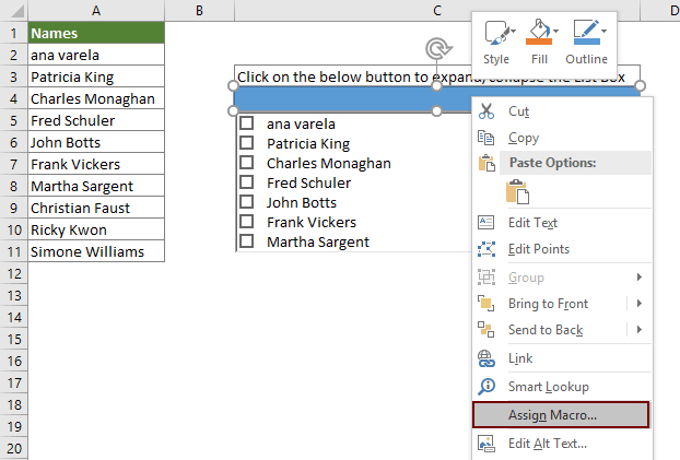
Как показано на скриншоте ниже, все имена в диапазоне A2:A11 текущего листа будут служить исходными данными для поля со списком, расположенного в ячейке C4. При нажатии на эту ячейку раскрывается список элементов, которые вы можете выбрать, а выбранные элементы будут отображаться в ячейке E4. Для достижения этого следуйте этим шагам:

A. Создайте поле со списком с исходными данными
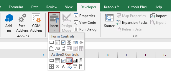
1. Нажмите Разработчик > Вставить > Поле со списком (Элемент управления ActiveX). Смотрите скриншот:
2. Нарисуйте поле со списком в текущем листе, щелкните его правой кнопкой мыши и выберите Свойства из контекстного меню.

3. В диалоговом окне Свойства вам нужно настроить следующее.
- 3.1 В поле ListFillRange введите исходный диапазон, который вы хотите отобразить в списке (здесь я ввожу диапазон A2:A11);
- 3.2 В поле ListStyle выберите 1 - fmListStyleOption;
- 3.3 В поле MultiSelect выберите 1 – fmMultiSelectMulti;
- 3.4 Закройте диалоговое окно Свойства. Смотрите скриншот:


B: Назовите ячейку, в которой будут находиться выбранные элементы
Если вам нужно вывести все выбранные элементы в определенную ячейку, например E4, выполните следующие действия.
1. Выберите ячейку E4, введите ListBoxOutput в поле имени и нажмите клавишу Enter.

C. Вставьте фигуру для вывода выбранных элементов
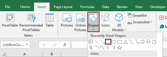
1. Нажмите Вставить > Фигуры > Прямоугольник. Смотрите скриншот:
2. Нарисуйте прямоугольник на вашем листе (здесь я рисую прямоугольник в ячейке C4). Затем щелкните правой кнопкой мыши по прямоугольнику и выберите Назначить макрос из контекстного меню.
3. В диалоговом окне Назначить макрос нажмите кнопку Создать.

4. В открывшемся окне Microsoft Visual Basic for Applications замените исходный код в окне Модуль на следующий VBA-код.
VBA-код: Создание списка с несколькими флажками
Sub Rectangle1_Click()
'Updated by Extendoffice 20200730
Dim xSelShp As Shape, xSelLst As Variant, I, J As Integer
Dim xV As String
Set xSelShp = ActiveSheet.Shapes(Application.Caller)
Set xLstBox = ActiveSheet.ListBox1
If xLstBox.Visible = False Then
    xLstBox.Visible = True
    xSelShp.TextFrame2.TextRange.Characters.Text = "Pickup Options"
    xStr = ""
    xStr = Range("ListBoxOutput").Value

    If xStr <> "" Then
         xArr = Split(xStr, ";")
    For I = xLstBox.ListCount - 1 To 0 Step -1
        xV = xLstBox.List(I)
        For J = 0 To UBound(xArr)
            If xArr(J) = xV Then
              xLstBox.Selected(I) = True
              Exit For
            End If
        Next
    Next I
    End If
Else
    xLstBox.Visible = False
    xSelShp.TextFrame2.TextRange.Characters.Text = "Select Options"
    For I = xLstBox.ListCount - 1 To 0 Step -1
        If xLstBox.Selected(I) = True Then
        xSelLst = xLstBox.List(I) & ";" & xSelLst
        End If
    Next I
    If xSelLst <> "" Then
        Range("ListBoxOutput") = Mid(xSelLst, 1, Len(xSelLst) - 1)
    Else
        Range("ListBoxOutput") = ""
    End If
End If
End Sub
Примечание: В коде Rectangle1 — это имя фигуры; ListBox1 — это имя поля со списком; Select Options и Pickup Options — это отображаемые тексты фигуры; а ListBoxOutput — это имя диапазона выходной ячейки. Вы можете изменить их по своему усмотрению.
5. Одновременно нажмите клавиши Alt + Q, чтобы закрыть окно Microsoft Visual Basic for Applications.
6. При нажатии на кнопку прямоугольника список будет сворачиваться или разворачиваться. Когда список развернут, выберите нужные элементы, отметив их галочками. Затем снова нажмите на прямоугольник, чтобы вывести все выбранные элементы в ячейку E4. Смотрите демонстрацию ниже:
7. И затем сохраните книгу как Книга Excel с поддержкой макросов для повторного использования кода в будущем.
Создайте выпадающий список с флажками с помощью удивительного инструмента
Устали от сложного программирования на VBA? Kutools для Excel делает создание выпадающих списков с флажками для удобного множественного выбора простым. Идеально подходит для опросов, фильтрации данных или динамических форм, этот удобный инструмент упрощает ваш рабочий процесс и экономит время.
1. Откройте лист, где вы установили выпадающий список проверки данных, нажмите Kutools > Выпадающий список > Включить расширенный выпадающий список. Затем нажмите Выпадающий список с флажками снова из Выпадающего списка. Смотрите скриншот:
 |  |
2. В диалоговом окне Добавить флажки в выпадающий список настройте следующее.
- 2.1) Выберите ячейки, содержащие выпадающий список;
- 2.2) В поле Разделитель введите разделитель, который вы будете использовать для разделения нескольких элементов;
- 2.3) Проверьте опцию Включить поиск при необходимости. (Если вы отметите эту опцию, позже можно будет выполнять поиск в выпадающем списке.)
- 2.4) Нажмите кнопку OK.


Теперь, когда вы нажмете на ячейку с выпадающим списком, появится окно списка, выберите элементы, отметив флажки для вывода в ячейку, как показано в демонстрации ниже.
Для получения дополнительной информации об этой функции посетите этот урок.
Kutools для Excel - Усильте Excel более чем 300 необходимыми инструментами. Наслаждайтесь постоянно бесплатными функциями ИИ! Получите прямо сейчас
В этой статье представлены два метода, которые помогут вам легко создать выпадающие списки с флажками в Excel. Вы можете выбрать тот, который вам больше нравится. Если вас интересуют другие советы и хитрости Excel, наш сайт предлагает тысячи уроков.
Связанные статьи:
Автозаполнение при вводе в выпадающем списке Excel
Если у вас есть выпадающий список проверки данных с большим количеством значений, вам нужно прокручивать список, чтобы найти нужное значение, или вводить слово целиком в поле списка. Если бы существовал метод автозаполнения при вводе первой буквы в выпадающем списке, всё стало бы проще. Этот урок предоставляет метод решения проблемы.
Создание выпадающего списка из другой книги в Excel
Очень просто создать выпадающий список проверки данных между листами внутри одной книги. Но если данные для проверки находятся в другой книге, что вы будете делать? В этом уроке вы узнаете, как создать выпадающий список из другой книги в Excel подробно.
Создание поискового выпадающего списка в Excel
Для выпадающего списка с большим количеством значений найти нужное не так просто. Ранее мы представили метод автозаполнения выпадающего списка при вводе первой буквы в поле списка. Помимо функции автозаполнения, вы также можете сделать выпадающий список доступным для поиска, чтобы повысить эффективность работы при поиске подходящих значений в выпадающем списке. Для создания поискового выпадающего списка попробуйте метод из этого урока.
Автоматическое заполнение других ячеек при выборе значений в выпадающем списке Excel
Допустим, вы создали выпадающий список на основе значений в диапазоне ячеек B8:B14. При выборе любого значения в выпадающем списке вы хотите, чтобы соответствующие значения в диапазоне ячеек C8:C14 автоматически заполнялись в выбранной ячейке. Для решения этой проблемы методы из этого урока помогут вам.
Лучшие инструменты для повышения продуктивности в Office
Повысьте свои навыки работы в Excel с помощью Kutools для Excel и ощутите эффективность на новом уровне. Kutools для Excel предлагает более300 расширенных функций для повышения производительности и экономии времени. Нажмите здесь, чтобы выбрать функцию, которая вам нужнее всего...
Office Tab добавляет вкладки в Office и делает вашу работу намного проще
- Включите режим вкладок для редактирования и чтения в Word, Excel, PowerPoint, Publisher, Access, Visio и Project.
- Открывайте и создавайте несколько документов во вкладках одного окна вместо новых отдельных окон.
- Увеличьте свою продуктивность на50% и уменьшите количество щелчков мышью на сотни ежедневно!
Все надстройки Kutools. Один установщик
Пакет Kutools for Office включает надстройки для Excel, Word, Outlook и PowerPoint, а также Office Tab Pro — идеально для команд, работающих в разных приложениях Office.
- Комплексный набор — надстройки для Excel, Word, Outlook и PowerPoint плюс Office Tab Pro
- Один установщик, одна лицензия — настройка занимает считанные минуты (MSI-совместимо)
- Совместная работа — максимальная эффективность между приложениями Office
- 30-дневная полнофункциональная пробная версия — без регистрации и кредитной карты
- Лучшее соотношение цены и качества — экономия по сравнению с покупкой отдельных надстроек