Перейти к основному содержанию

Как вывести соответствующее название наивысшего балла в Excel?

Предположим, у меня есть диапазон данных, который содержит два столбца - столбец имени и соответствующий столбец оценки, теперь я хочу получить имя человека, который набрал наибольшее количество баллов. Есть ли какие-нибудь хорошие способы быстро решить эту проблему в Excel?

Отображение соответствующего имени наивысшего балла с формулами


стрелка синий правый пузырь Отображение соответствующего имени наивысшего балла с формулами

Чтобы получить имя человека, набравшего наибольшее количество баллов, следующие формулы могут помочь вам получить результат.

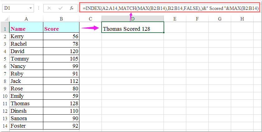
Пожалуйста, введите эту формулу: =INDEX(A2:A14,MATCH(MAX(B2:B14),B2:B14,FALSE),)&" Scored "&MAX(B2:B14) в пустую ячейку, где вы хотите отобразить имя, а затем нажмите Enter ключ, чтобы вернуть результат следующим образом:

отображаемое имя документа наивысший балл 1

Ноты:

1. В приведенной выше формуле A2: A14 это список имен, из которого вы хотите получить имя, и B2: B14 это список очков.

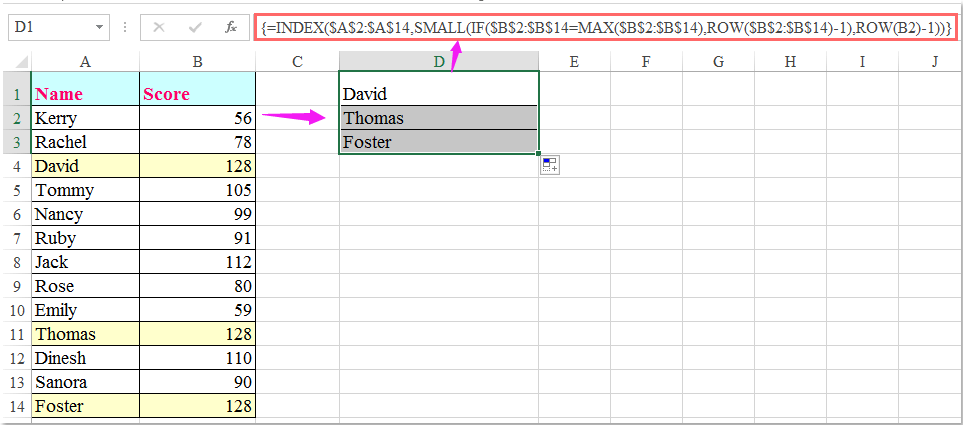
2. Приведенная выше формула может получить имя только в том случае, если существует несколько имен, имеющих одинаковые наивысшие оценки. Чтобы получить все имена, получившие наибольшее количество баллов, следующая формула массива может оказать вам услугу.

Введите эту формулу:

=INDEX($A$2:$A$14,SMALL(IF($B$2:$B$14=MAX($B$2:$B$14),ROW($B$2:$B$14)-1),ROW(B2)-1)), а затем нажмите Shift + Ctrl + Enter вместе, чтобы отобразить имя, затем выберите ячейку с формулой и перетащите дескриптор заполнения вниз, пока не появится значение ошибки, все имена, получившие наивысший балл, отображаются, как показано на снимке экрана ниже:

отображаемое имя документа наивысший балл 2

Лучшие инструменты для офисной работы

🤖 Kutools AI Помощник: Революционный анализ данных на основе: Интеллектуальное исполнение   |  Генерировать код  |  Создание пользовательских формул  |  Анализ данных и создание диаграмм  |  Вызов функций Kutools...
Популярные опции: Найдите, выделите или определите дубликаты   |  Удалить пустые строки   |  Объедините столбцы или ячейки без потери данных   |   Раунд без формулы ...
Супер поиск: Множественный критерий VLookup    VLookup с несколькими значениями  |   VLookup по нескольким листам   |   Нечеткий поиск ....
Расширенный раскрывающийся список: Быстрое создание раскрывающегося списка   |  Зависимый раскрывающийся список   |  Выпадающий список с множественным выбором ....
Менеджер столбцов: Добавить определенное количество столбцов  |  Переместить столбцы  |  Переключить статус видимости скрытых столбцов  |  Сравнить диапазоны и столбцы ...
Рекомендуемые функции: Сетка Фокус   |  Просмотр дизайна   |   Большой Формулный Бар    Менеджер книг и листов   |  Библиотека ресурсов (Авто текст)   |  Выбор даты   |  Комбинировать листы   |  Шифровать/дешифровать ячейки    Отправлять электронные письма по списку   |  Суперфильтр   |   Специальный фильтр (фильтровать жирным шрифтом/курсивом/зачеркиванием...) ...
15 лучших наборов инструментов12 Текст Инструменты (Добавить текст, Удалить символы, ...)   |   50+ График Тип (Диаграмма Ганта, ...)   |   40+ Практических Формулы (Рассчитать возраст по дню рождения, ...)   |   19 Вносимые Инструменты (Вставить QR-код, Вставить изображение из пути, ...)   |   12 Конверсия Инструменты (Числа в слова, Конверсия валюты, ...)   |   7 Слияние и разделение Инструменты (Расширенные ряды комбинирования, Разделить клетки, ...)   |   ... и более

Улучшите свои навыки работы с Excel с помощью Kutools for Excel и почувствуйте эффективность, как никогда раньше. Kutools for Excel предлагает более 300 расширенных функций для повышения производительности и экономии времени.  Нажмите здесь, чтобы получить функцию, которая вам нужна больше всего...

Описание


Вкладка Office: интерфейс с вкладками в Office и упрощение работы

  • Включение редактирования и чтения с вкладками в Word, Excel, PowerPoint, Издатель, доступ, Visio и проект.
  • Открывайте и создавайте несколько документов на новых вкладках одного окна, а не в новых окнах.
  • Повышает вашу продуктивность на 50% и сокращает количество щелчков мышью на сотни каждый день!
Comments (17)
No ratings yet. Be the first to rate!
This comment was minimized by the moderator on the site
Hi sir, I tried this method, But the problem is if top two students have the same score when I look for the highest 3 one student's name alone is repeated twice with the same score instead of second student's name. How to solve this.
This comment was minimized by the moderator on the site
Hello, Divyanathan
Maybe the following array formula can help you:

=IFERROR(INDEX(A:A,SUM(IF(($B$2:$B$100+ROUND(0.1/ROW($B$2:$B$100),5))=LARGE($B$2:$B$100+ROUND(0.1/ROW($B$2:$B$100),5),ROW(A1)),ROW($B$2:$B$100)))),"")


Note: After inserting the formula, please press Ctrl + Shift + Enter keys together to get the first result, and then drga this formula cell down to get the largest n results as you need.

Please have a try, hope it can help you!
This comment was minimized by the moderator on the site
Hola disculpa me podrías apoyar para sacar la formula o otro tipo de dato que me pueda dar el nombre del tota de un resultado?

explico tengo una tabla con 4 nombres diferentes distribuidos en las celdas C3,D3,E3 y F3 de las cuales cada celda mencionada tiene rangos de productos ejemplo: detergentes
y cada celda mencionada tiene precios diferentes.
en el resultado que debo de mostrar es el valor mínimo de precio de cada detergente de las celdas ya mencionadas arriba, y a lo que quiero llegar es que indique una formula o un dato que indique que en cada resultado a la derecho me indique el nombre del valor de resultado.
muestro un ejemplo mas especifico: en la celda <C3> tiene un nombre de insumos, en la celda C4 hasta C120 están los precios de cada detergente que maneja la celda C3, en la celda <D3> esta un nombre de biodetergentes, y mismo proceso la celda D4 hasta D120 están los precios en la celda G4 se encuentra el resultado del valor mínimo de estos dos nombres (insumos-biodetergentes) teniendo el valor menor el de nombre de insumos. ahora en la celda H4 quiero que me aparezca el nombre del valor de resultado en este caso que me aparezca el nombre de "insumos" como puedo hacer para que me aparezca este nombre? espero me allá podido dar a entender de lo que requiero
muchas gracias por su atención
saludos cordiales.
This comment was minimized by the moderator on the site
ik heb het ook geprobeerd met alle dezelfde gegevens zoals in het voorbeeld maar het werkt totaal niet
This comment was minimized by the moderator on the site
Hello jac, Sorry to hear that. As I have answered in the below comment, the two formulas work great for me. And I have been wondering why the formulas aren't working for the readers. There are two reasons that can lead to the malfunction of the second formula. 
First, if you are using Excel versions before Excel 2020, then you must enter the formula =INDEX($A$2:$A$14,SMALL(IF($B$2:$B$14=MAX($B$2:$B$14),ROW($B$2:$B$14)-1),ROW(B2)-1)) via pressing Ctrl + Shift + Enter keys together.
Second, When you get the first result, remember to select the formula cell and drag the fill handle down until error value appears. So all the other results will be returned.
And as you can see in the screenshots below, the two formulas are working fine for me.  Hope my solution works. Have a nice day.
Sincerely,Mandy
This comment was minimized by the moderator on the site
bullshitdoes not work
This comment was minimized by the moderator on the site
Hello,
Sorry to hear that. But I did tried the two formulas in the article and both of them works perfectly. Please see the screenshots I uploaded here. And we would love to solve the problem for you if you can provide the details of the problem. Looking forward to your reply.Sincerely,Mandy
This comment was minimized by the moderator on the site
Trying to do the same thing but with the minimum score in Microsoft sheets. I swapped max for min as below and it didn't work =INDEX($A$2:$A$14,SMALL(IF($B$2:$B$14=MIN($B$2:$B$14),ROW($B$2:$B$14)-1),ROW(B2)-1))
This comment was minimized by the moderator on the site
Hi. This formula was exactly what I was looking for. However is there a way do this with the lowest Score but above 0 (in my case £00.00) I removed the bit of formula that displays the amount as only needed the Name and comment.I changed the MAX for MIN but there are a few entries at 0 (£00.00) and formula displays the name for the first of the '0' entries
This comment was minimized by the moderator on the site
Hello, Nigel,To lookup the lowest value above 0, you should apply the below array formula:After entering the formula, please remember to press Ctrl + Shift + Enter keys together to get the correct result.=INDEX(A2:A8,MATCH(MIN(IF(B2:B8>0,B2:B8)),B2:B8,0))&" Scored "&MIN(IF(B2:B8>0,B2:B8))
Please try, hope it can help you!
This comment was minimized by the moderator on the site
How do you find the second highest student? Please help me :( I only get the name of Thomas.
This comment was minimized by the moderator on the site
How do you find the second highest student?
This comment was minimized by the moderator on the site
How would you show two names if the high scores match?
This comment was minimized by the moderator on the site
Hello, Chris,
To get all names if there are multiple high scores match, the second formula in this article can do you a favor.
Please try it, thank you!
This comment was minimized by the moderator on the site
How would you get the matching numbers with the corresponding names to display horizontally?
There are no comments posted here yet
Load More
Please leave your comments in English
Posting as Guest
×
Rate this post:
0   Characters
Suggested Locations