Как объединить ячейки, если такое же значение существует в другом столбце Excel?
Как показано на снимке экрана ниже, если вы хотите объединить ячейки во втором столбце на основе тех же значений в первом столбце, вы можете использовать несколько методов. В этой статье мы представим три способа выполнения этой задачи.

Объединить ячейки, если одинаковое значение, с формулами и фильтром
Следующие формулы помогают объединить содержимое соответствующих ячеек в столбце на основе того же значения в другом столбце.
1. Выберите пустую ячейку помимо второго столбца (здесь мы выбираем ячейку C2), введите формулу = ЕСЛИ (A2 <> A1, B2, C1 & "," & B2) в строку формул, а затем нажмите Enter .

2. Затем выберите ячейку C2 и перетащите маркер заполнения вниз к ячейкам, которые необходимо объединить.

3. Введите формулу = ЕСЛИ (A2 <> A3, СЦЕПИТЬ (A2, "," "", C2, "" ""), "") в ячейку D2 и перетащите маркер заполнения вниз до остальных ячеек.

4. Выберите ячейку D1 и щелкните Данные > ФИЛЬТР. Смотрите скриншот:

5. Щелкните стрелку раскрывающегося списка в ячейке D1, снимите флажок (Пробелы) поле, а затем щелкните OK .

Вы можете видеть, что ячейки объединены, если значения первого столбца совпадают.

Внимание: Для успешного использования приведенных выше формул одни и те же значения в столбце A должны быть непрерывными.
Легко объединять ячейки, если одинаковое значение с Kutools for Excel (несколько кликов)
Описанный выше метод требует создания двух вспомогательных столбцов и включает несколько шагов, что может быть неудобно. Если вы ищете более простой способ, рассмотрите возможность использования Расширенные ряды комбинирования инструмент из Kutools for Excel. Всего за несколько кликов эта утилита позволяет вам объединять ячейки, используя определенный разделитель, что делает процесс быстрым и беспроблемным.
Функции: Перед применением этого инструмента установите Kutools for Excel в первую очередь. Перейти к бесплатной загрузке сейчас.
- Выберите диапазон, который вы хотите объединить;
- Установите столбец с теми же значениями, что и Основной ключ колонка.
- Укажите разделитель для объединения ячеек.
- Нажмите OK.
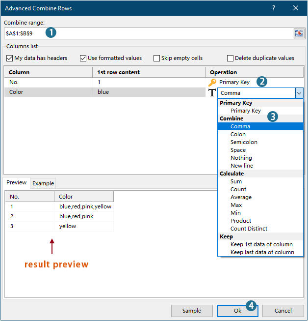
Результат

- Чтобы применить эту функцию, пожалуйста, скачайте и установите Kutools для Excel первый.
- Чтобы узнать больше об этой функции, ознакомьтесь с этой статьей: Быстро объединяйте одинаковые значения или повторяющиеся строки в Excel
Объединить ячейки, если то же значение с кодом VBA
Вы также можете использовать код VBA для объединения ячеек в столбце, если такое же значение существует в другом столбце.
1. Нажмите другой + F11 , чтобы открыть Приложения Microsoft Visual Basic окно.
2. в Приложения Microsoft Visual Basic окна, нажмите Вставить > Модули. Затем скопируйте и вставьте приведенный ниже код в Модули окно.
Код VBA: объединение ячеек при одинаковых значениях
Sub ConcatenateCellsIfSameValues()
	Dim xCol As New Collection
	Dim xSrc As Variant
	Dim xRes() As Variant
	Dim I As Long
	Dim J As Long
	Dim xRg As Range
	xSrc    = Range("A1", Cells(Rows.Count, "A").End(xlUp)).Resize(, 2)
	Set xRg = Range("D1")
	On Error Resume Next
	For I = 2 To UBound(xSrc)
		xCol.Add xSrc(I, 1), TypeName(xSrc(I, 1)) & CStr(xSrc(I, 1))
	Next I
	On Error GoTo 0
	ReDim xRes(1 To xCol.Count + 1, 1 To 2)
	xRes(1, 1) = "No"
	xRes(1, 2) = "Combined Color"
	For I = 1 To xCol.Count
		xRes(I + 1, 1) = xCol(I)
		For J = 2 To UBound(xSrc)
			If xSrc(J, 1) = xRes(I + 1, 1) Then
				xRes(I + 1, 2) = xRes(I + 1, 2) & ", " & xSrc(J, 2)
			End If
		Next J
		xRes(I + 1, 2) = Mid(xRes(I + 1, 2), 2)
	Next I
	Set xRg = xRg.Resize(UBound(xRes, 1), UBound(xRes, 2))
	xRg.NumberFormat = "@"
	xRg = xRes
	xRg.EntireColumn.AutoFit
End SubЗаметки:
3. нажмите F5 ключ для запуска кода, то вы получите объединенные результаты в указанном диапазоне.

Легко объединять ячейки, если то же значение с Kutools for Excel
Лучшие инструменты для офисной работы
Улучшите свои навыки работы с Excel с помощью Kutools for Excel и почувствуйте эффективность, как никогда раньше. Kutools for Excel предлагает более 300 расширенных функций для повышения производительности и экономии времени. Нажмите здесь, чтобы получить функцию, которая вам нужна больше всего...
")
Вкладка Office: интерфейс с вкладками в Office и упрощение работы
- Включение редактирования и чтения с вкладками в Word, Excel, PowerPoint, Издатель, доступ, Visio и проект.
- Открывайте и создавайте несколько документов на новых вкладках одного окна, а не в новых окнах.
- Повышает вашу продуктивность на 50% и сокращает количество щелчков мышью на сотни каждый день!
")