Как найти первую или последнюю пятницу каждого месяца в Excel?
Обычно пятница является последним рабочим днем месяца. Как можно найти первую или последнюю пятницу на основе заданной даты в Excel? В этой статье мы проведем вас через использование двух формул для поиска первой или последней пятницы каждого месяца.
Найти первую пятницу месяца
Найти последнюю пятницу месяца
Найти первую пятницу месяца
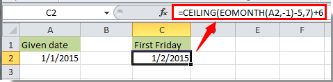
Например, заданная дата 01.01.2015 находится в ячейке A2, как показано на скриншоте ниже. Если вы хотите найти первую пятницу месяца на основе заданной даты, выполните следующие действия.
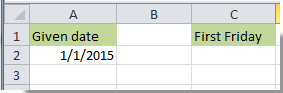
1. Выберите ячейку для отображения результата. Здесь мы выбираем ячейку C2.
2. Скопируйте и вставьте следующую формулу в нее, затем нажмите клавишу Enter.
=ОКРВВЕРХ(КОНЕЦМЕСЯЦА(A2;-1)-5;7)+6
Примечания:
Найти последнюю пятницу месяца
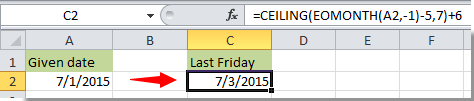
Заданная дата 01.01.2015 находится в ячейке A2. Для того чтобы найти последнюю пятницу этого месяца в Excel, выполните следующие действия.
1. Выберите ячейку, скопируйте в неё следующую формулу и нажмите клавишу Enter, чтобы получить результат.
=ДАТА(ГОД(A2);МЕСЯЦ(A2)+1;0)+ОСТАТ(-ДЕНЬНЕД(ДАТА(ГОД(A2);МЕСЯЦ(A2)+1;0);2)-2;-7)

Примечание: Вы можете изменить A2 в формуле на ссылочную ячейку вашей заданной даты.
Связанные статьи:
- Как найти наименьшие и наибольшие 5 значений в списке в Excel?
- Как найти или проверить, открыт ли конкретный файл книги в Excel?
- Как узнать, используется ли ячейка в другой ячейке в Excel?
- Как найти ближайшую к сегодняшнему дню дату в списке в Excel?
Лучшие инструменты для повышения продуктивности в Office
Повысьте свои навыки работы в Excel с помощью Kutools для Excel и ощутите эффективность на новом уровне. Kutools для Excel предлагает более300 расширенных функций для повышения производительности и экономии времени. Нажмите здесь, чтобы выбрать функцию, которая вам нужнее всего...
Office Tab добавляет вкладки в Office и делает вашу работу намного проще
- Включите режим вкладок для редактирования и чтения в Word, Excel, PowerPoint, Publisher, Access, Visio и Project.
- Открывайте и создавайте несколько документов во вкладках одного окна вместо новых отдельных окон.
- Увеличьте свою продуктивность на50% и уменьшите количество щелчков мышью на сотни ежедневно!
Все надстройки Kutools. Один установщик
Пакет Kutools for Office включает надстройки для Excel, Word, Outlook и PowerPoint, а также Office Tab Pro — идеально для команд, работающих в разных приложениях Office.
- Комплексный набор — надстройки для Excel, Word, Outlook и PowerPoint плюс Office Tab Pro
- Один установщик, одна лицензия — настройка занимает считанные минуты (MSI-совместимо)
- Совместная работа — максимальная эффективность между приложениями Office
- 30-дневная полнофункциональная пробная версия — без регистрации и кредитной карты
- Лучшее соотношение цены и качества — экономия по сравнению с покупкой отдельных надстроек